Introduction

Knowing all about the software system we are developing is valuable, but too often a rare situation we are facing today. In times of software development experts shortages and stressful software projects, high turnover in teams leads quickly to lost knowledge about the source code (<scrumcasm>And who needs to document? We do Scrum!</scrumcasm>).

I already did some calculations of the knowledge distribution of software systems based on Adam Tornhill marvelous ideas in “Your Code as a Crime Scene” (publisher’s site, but my recommendation is to get the newer book). It really did its job. But after my experiences from a Subversion to Git migration (where I, who guessed it, ensured the quality of the migrated data 🙂 ), I’ve found another neat idea for another model to find lost knowledge that feels more naturally what we do as developers.

The Idea

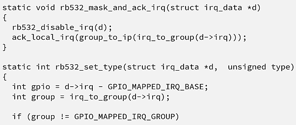
How do you define knowledge about your code? We could get into a deep philosophical discussion about what knowledge is and if there is such a thing as knowledge (invite me to a beer if you want to start this discourse ;-)). But let’s look at it from a developer’s point of view: E. g. in my case, every time I want to know who could possibly know something about a code line, for example, for this piece of code (the meaning of the source code is irrelevant here),

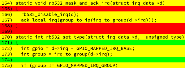
I’m catching myself using the blame appraisal features of version control systems heavily. This feature calculates the latest change for each line. The resulting view gives me very helpful hints about what changes in a source code line happened recently

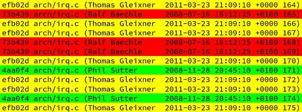
with plenty of additional information about who and when this change occurred.

With these results, I can take a look at the author of the code and the timestamp of the code change. This gives me enough hints about the circumstances in which the code change happened and if the the original author could still possibly know anything about the source code line. Here, I’m using Eagleson’s law as a heuristic:

Eagleson’s Law: Any code of your own that you haven’t looked at for six or more months might as well have been written by someone else.

— Programming Wisdom (@CodeWisdom) Dezember 10th 2017

If the code change is older than six months, it’s very likely that the knowledge about the source code line is lost completely.

So there we have it: A reasonable model of code knowledge! If we would have this information for all source code files of our software project, we would be able to identify the areas in our software system with lost knowledge (and find out, if we are screwed in a challenging situation!).

So, let’s get the data we need for this analysis!

Number Crunching (aka Data Preparation)

Note: Click here if you can’t see bad data: Take me to the actual analysis!

Getting the data is straightforward: We just need a software system that used a version control system like Git for managing the code changes. I choose the GitHub mirror repository of the Linux kernel for this demonstration. The reason? It’s big! In this repo, we have a snapshot of the last 13 years of Linux kernel development at our hand with over 750000 commits and some millions lines of source code.

We can get our hands on the necessary data with the git blame command that we execute for each source code file in the repository. There is a nice little bash command that makes this happen for us:

find . -type d -name ".git" -prune -o -type f \( -iname "*.c" -o -iname "*.h" \) | xargs -n1 git blame -w -f >> git_blame.log

It first finds all C programming language source code files (.h header files as well as th.c program files) and retrieves the git blame information for each source code line in each file. This information includes

the sha id of the commit
the relative path of the file
the name of the author
the commit timestamp
the source line number
the source code line itself

The result is stored in a plain text file named git_blame.log.

At this point you might ask: “OK, wait a minute: 13 years of development efforts, with around 750000 commits and (spoiler alert!) 10235 source code files that sum up to 5.6 millions lines of code. Are you insane?”

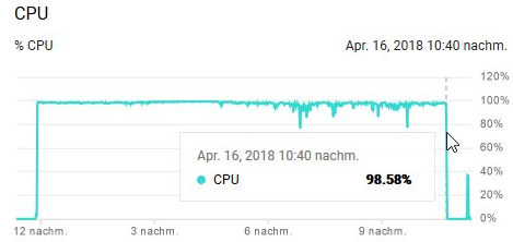
Well kind of. I hadn’t thought that retrieving the data set would take so long. But in the end, I didn’t care because I did the calculation on a Google Cloud Compute Engine, which was pretty busy for 11 hours on a n1-standard-1 CPU (which cost me 30 cents, donations welcome :-D):

The result was a 3 GB big log file that I’ve packed and downloaded to my computer. And this is where we start the first part our analysis with Python and Pandas!

Wrangling the raw data

First, I want to create a nice little comma separated file with only the data we need for later analysis. This is why we first take the raw data and transform it to something we can call a decent data set.

I have my experiences with old and big repositories, so I know that it’s not going to be easy to read in such a long runner. The nice and bad thing at the same time is, that the Linux kernel was developed internationally. This means fun with character encodings! It seems that every nation has its own way of encoding their special character sets. Especially when working with the author’s names, it’s really a PITA. You simply cannot read in the dataset with standard means. The universal weapon for this is to import data into a Pandas DataFrame with the encoding latin-1 which seems to don’t care if there are some weird characters in the data (but unfortunately, screwing up foreign characters, which is not so important in our case).

Additionally, there is no good format for outputting the Git blame log in a way, that it’s easy to process. There are some flags for machine-friendly output, but these are multi-line formats (which are…not very nice to work within Pandas). So in these cases, I like to eat get my data in a very raw format. There is this other trick to use a non-used separator (I prefer \u0012) that makes Pandas reading in a text file row by row in one single column.

So let’s do this!

import pandas as pd

PATH = r"C:\Users\Markus\Downloads\linux_blame_temp.tar.gz"
blame_raw = pd.read_csv(PATH, encoding="latin-1", sep="\u0012", names=["raw"])
blame_raw.head()

After around 30 seconds, we read in our 3 GB Git blame log (I think this is kind of okayish). Maybe you’re wondering why this takes so long. Well, let’s see how many entries are in our dataset.

len(blame_raw)

5665949

There are 5.6 million entries (= source code lines) that needed to be read in.

In the next code cell, we extract all the data from the raw column into a new DataFrame called blame. We just need to figure out the right regular expression for this and we are fine. In this step, we also exclude the source code of the blame log because we actually don’t need this information for our knowledge loss calculation.

As always when working with string data, this needs time.

blame = \
  blame_raw.raw.str.extract(
      "(?P<sha>.*?) (?P<path>.*?) \((?P<author>.* ?) (?P<timestamp>[0-9]{4}-[0-9]{2}-[0-9]{2} [0-9]{2}:[0-9]{2}:[0-9]{2} .[0-9]{4}) *(?P<line>[0-9]*)\) .*",
      expand=True)
blame.head()

But after a minute we have the data in a nice new DataFrame, too.

Fixing missing / wrong entries

In the next step, we have to face some missing data. I think I did a mistake by executing the bash command in the wrong directory. This could explain why there are some missing values. We simply drop the missing data but log the number of the missed entries to make sure we are working reproducible.

has_null_value = blame.isnull().any(axis=1)
dropped_entries = blame[has_null_value]
blame = blame[~has_null_value]
dropped_entries

So we lost the first non-sense line (because of my mistake), thus the second entry for the first Git blame result as well as the last line (which is negligible in our case). For completeness reasons, let’s add the first line manually (because I want to share a clean dataset with you as well!).

blame.head()

We take the second line and alter the data so that we have the first line again (as long as we have good and comprehensible reasons for this, I find this approach OK here).

first_line = blame.loc[2].copy()
first_line.line = 1
first_line

sha                        889d0d42667c9
path         drivers/scsi/bfa/bfad_drv.h
author                Anil Gurumurthy   
timestamp      2015-11-26 03:54:45 -0500
line                                   1
Name: 2, dtype: object

We transform our single entry back into a DataFrame, transpose the data and concatenate our blame DataFrame to it.

blame = pd.concat([pd.DataFrame(first_line).T, blame])
blame.head()

After this, we do some housekeeping of the data:

We fix the comma-separated values in the author’s column by replacing all commas with a semicolon because we want to use the comma as separator for our comma-separated values (CSV) file
We also change the data type of the timestamp from a string to a TimeStamp to check it’s data quality

To improve performance, we first convert both columns into Categorical data to enable working with references instead of manipulating the values for all entries. It the end, this means that the same values need to be changed and converted only once.

blame.author = pd.Categorical(blame.author)
blame.author = blame.author.str.replace(",", ";")

blame.timestamp = pd.Categorical(blame.timestamp)
blame.timestamp = pd.to_datetime(blame.timestamp)
blame.info()

<class 'pandas.core.frame.DataFrame'>
Int64Index: 5665947 entries, 2 to 5665947
Data columns (total 5 columns):
sha          object
path         object
author       object
timestamp    datetime64[ns]
line         object
dtypes: datetime64[ns](1), object(4)
memory usage: 259.4+ MB

This operation takes a minute, but we have now a decent dataset that we can use further on.

Next, we take a look at another possible area of errors: The timestamp column.

blame.timestamp.describe()

count                 5665947
unique                  92466
top       2005-04-16 22:20:36
freq                   836898
first     2002-04-09 19:14:34
last      2018-04-11 17:26:09
Name: timestamp, dtype: object

Apparently, the Linux Git repository has also some issues with timestamps. The (still) top occurring timestamp is the initial commit of Linux Torvalds in April 2005. There is nothing we can do about that than mention that here. But there are also changes that are older than that. This is an error caused by wrong clock configurations from a few developers. This leaves us with no other choice with either deleting the entries with that data or assigning them to the initial commits.

Because in our case, we want to have a complete dataset, we choose the second option. Not quite clean, but the best decision we can make in our situation. And always remember:

All models are wrong but some are useful

— George Box

Let’s find the initial commit of Linux Torvalds.

initial_commit = blame[blame.author == "Linus Torvalds"].timestamp.min()
initial_commit

Timestamp('2005-04-16 22:20:36')

We keep track of all wrong timestamps and set those to the initial commit timestamp.

is_wrong_timestamp = blame.timestamp < initial_commit
wrong_timestamps = blame[is_wrong_timestamp]
blame.timestamp = blame.timestamp.clip(initial_commit)
len(wrong_timestamps)

4955

Further, we convert the timestamp column to an integer (into nanoseconds until UNIX epoch) to save some storage and to enable efficient timestamp transformation when reading the data in later on.

blame.timestamp = blame.timestamp.astype('int64')
blame.head()

Last, we store the result in a gzipped CSV file as an immediate result.

blame.to_csv("C:/Temp/linux_blame.gz", encoding='utf-8', compression='gzip', index=None)

All right, the ugly work finished! Let’s get some insights!

Analyzing the knowledge around the Linux kernel

Importing the dataset (again)

First, we reimport our newly created data set to check if it’s as expected (this is where you can start your own analysis with the dataset, too. You can download it here [21 MB])

git_blame = pd.read_csv("C:/Temp/linux_blame.gz")
git_blame.head()

Let’s first have a look at what we’ve got here now.

git_blame.info(memory_usage='deep')

<class 'pandas.core.frame.DataFrame'>
RangeIndex: 5665947 entries, 0 to 5665946
Data columns (total 5 columns):
sha          object
path         object
author       object
timestamp    int64
line         int64
dtypes: int64(2), object(3)
memory usage: 1.4 GB

We have our 5.6 million Git blame log entries that are stored in memory with 1.3 GB. We need (as always) do some data wrangling by applying some data conversions. In this case, we convert the sha, path, and author columns to Categorical data (as mentioned above, because of performance reasons).

git_blame.sha = pd.Categorical(git_blame.sha)
git_blame.path = pd.Categorical(git_blame.path)
git_blame.author = pd.Categorical(git_blame.author)
git_blame.info(memory_usage='deep')

<class 'pandas.core.frame.DataFrame'>
RangeIndex: 5665947 entries, 0 to 5665946
Data columns (total 5 columns):
sha          category
path         category
author       category
timestamp    int64
line         int64
dtypes: category(3), int64(2)
memory usage: 141.8 MB

This bring down the data in memory down to 140 MB. Next, we convert the timestamp from nanoseconds to real TimeStamp data.

git_blame.timestamp = pd.to_datetime(git_blame.timestamp)
git_blame.info(memory_usage='deep')

<class 'pandas.core.frame.DataFrame'>
RangeIndex: 5665947 entries, 0 to 5665946
Data columns (total 5 columns):
sha          category
path         category
author       category
timestamp    datetime64[ns]
line         int64
dtypes: category(3), datetime64[ns](1), int64(1)
memory usage: 141.8 MB

This didn’t improve the memory usage further, but we now have a nice TimeStamp data type in the timestamp column that makes working with time-based data easy as pie.

Calculate basic data

Alright, time to get some overview of our dataset.

How many files are we talking about?

git_blame.path.nunique()

10235

What is the biggest file?

git_blame[git_blame.line == git_blame.line.max()]

For which source file can we ask most of the authors?

authors_per_file = git_blame.groupby(['path']).author.nunique()
authors_per_file[authors_per_file == authors_per_file.max()]

path
drivers/pci/quirks.c    145
Name: author, dtype: int64

And for how many source files is only one author coding?

authors_per_file[authors_per_file == 1].count()

1903

Let’s do some analysis regarding knowledge.

Active knowledge carrier

Let’s see (after Eagleson’s law) which developers changes most of the source code files in the last six months.

We first create the timestamp six month ago

six_months_ago = pd.Timestamp('now') - pd.DateOffset(months=6)
six_months_ago

Timestamp('2017-10-24 12:59:06.271767')

and create a new column named knowing to get the information for the more recent changes.

git_blame['knowing'] = git_blame.timestamp >= six_months_ago
git_blame.head()

Let’s have look at the ratio of known code to unknown code (= code older than six months).

%matplotlib inline
git_blame['knowing'].value_counts().plot.pie(label="")
print(git_blame['knowing'].mean())

0.0399161870028

Phew…only 4% of the code changes occured in the last six months. This is what I would call “challenging”.

We need to take action! So let’s find out which developers did the most changes (maybe sending them some presents can help here :-)).

top10 = git_blame[git_blame.knowing].author.value_counts().head(10)
top10

Anirudh Venkataramanan     18790
Yasunari Takiguchi         11041
Tomer Tayar                 4959
Linus Walleij               3551
Bryan Whitehead             3364
Edward Cree                 3068
Tim Harvey                  2818
Rahul Lakkireddy            2811
Mauro Carvalho Chehab       2761
Yong Zhi                    2474
Name: author, dtype: int64

Actively developed components

We can also find out in which code areas is still knowledge available and which ones are the “no-go areas” in our code base. For this, we aggregate our data on a higher level by looking at the source code at the component level. In the Linux kernel, we can easily create this view because mostly, the first two parts of the source code path indicate the component.

git_blame.path.value_counts().head()

drivers/media/dvb-frontends/drx39xyj/drxj_map.h    15055
drivers/isdn/hardware/eicon/message.c              14954
drivers/net/ethernet/sfc/mcdi_pcol.h               14534
drivers/net/ethernet/intel/i40e/i40e_main.c        14484
drivers/staging/rdma/hfi1/chip.c                   13914
Name: path, dtype: int64

We need to do some string magic to fetch only the first two parts.

git_blame['component'] = git_blame.path.str.split("/", n=2).str[:2].str.join(":")
git_blame.head()

After this, we can group our data by the new component column and calculate the ratio of known and not known code by using the mean method.

knowledge_per_component = git_blame.groupby('component').knowing.mean()
knowledge_per_component.head()

component
arch:arc     0.000000
arch:arm     0.000118
arch:i386    0.000000
arch:ia64    0.000000
arch:mips    0.000000
Name: knowing, dtype: float64

We can create a little visualization of the top 10 known parts by sorting the “knowledge” for a component and plotting a a bar chart.

knowledge_per_component.sort_values(ascending=False).head(10).plot.bar();

Discussion
We see that in the last six months, some developers worked heavily on the SoundWIRE capabilities of Linux. So there might be still the chance to find some author how knows everything about this component. We also see some minor changes in other areas.

Top 10 No-Go Areas

But where are the no-go areas in the Linux kernel project? That means which are the oldest parts of the system (where it is also likely that nobody knows anything all)? For this, we create a new column named age and calculate the difference between today and the timestamp column.

git_blame['age'] = pd.Timestamp('now') - git_blame.timestamp
git_blame.head()

We need a little helper method mean that calculates the mean timestamp delta for each component (for reasons unknown, it doesn’t work with the standard mean() method of Pandas).

def mean(x):
    return x.mean()

mean_age_per_component = git_blame.groupby('component').age.agg([mean, 'count'])
mean_age_per_component.head()

Again, we sort the resulting values and just take the first 10 rows with the oldest mean age.

top10_no_go_areas = mean_age_per_component.sort_values('mean', ascending=False).head(10)
top10_no_go_areas

Discussion
The result isn’t as bad as it looks at the first glance: The oldest parts of the system are archaic computer architectures like SPARC64 (arch:sparc64), x86 (arch:i386), Itanium (arch:ia64) or PowerPC (arch:powerpc). So this is negligible because these architectures are dead anyways.

We also got lucky with the component drivers:isdn, where we have around 184917 lines of rotted code. In the age of glass fiber, we surely don’t need any improvements in the ISDN features of Linux.

Unfortunately, I’m not a Linux expert, so I can’t judge the impact of the lost knowledge in the component drivers:usb as well as the remaining components.

Conclusion

OK, I hope you’ve enjoyed this little longer analysis of the Linux Git repository! We’ve created a big data set right from the origin, wrangled our way through the Git blame data to finally get some insights into the parts of the Linux kernel, where knowledge is most likely lost forever.

One remark on the meta-level: Did I exaggerate by taking the complete Git blame log from one of the biggest open-source projects out there? Absolutely! Couldn’t I’ve just exported the really needed sub data set for the analysis? For Sure! But besides showing you what you can find out with this dataset, I wanted to show you that it’s absolutely no problem to work with a 3 GB data set like we had. You don’t need any Big Data tooling or set up a cluster for computations. With Pandas, e. g. I can execute this analysis on my six-year-old notebook. Period!

	raw
0	linux_blame_temp.log
1	NaN
2	889d0d42667c9 drivers/scsi/bfa/bfad_drv.h (Ani…
3	889d0d42667c9 drivers/scsi/bfa/bfad_drv.h (Ani…
4	7725ccfda5971 drivers/scsi/bfa/bfad_drv.h (Jin…

	sha	path	author	timestamp	line
0	NaN	NaN	NaN	NaN	NaN
1	NaN	NaN	NaN	NaN	NaN
5665948	NaN	NaN	NaN	NaN	NaN

	mean	count
component
arch:arc	1143 days 15:32:24.462724	311
arch:arm	2875 days 11:38:42.770369	8507
arch:i386	4638 days 09:16:08.708604	6561
arch:ia64	4508 days 07:58:41.529968	298
arch:mips	2804 days 05:20:25.948138	192

	mean	count
component
arch:sparc64	4744 days 21:49:04.517812	530
arch:i386	4638 days 09:16:08.708604	6561
drivers:usb	4588 days 19:48:11.197162	9163
arch:ia64	4508 days 07:58:41.529968	298
drivers:parisc	4484 days 04:17:20.798802	12765
drivers:sn	4439 days 07:15:56.174876	843
include:asm-arm	4426 days 18:19:32.521176	129
drivers:isdn	4325 days 08:35:42.713375	184917
arch:powerpc	4313 days 05:14:50.021728	1973
drivers:message	4286 days 16:32:08.297454	35594

feststelltaste

Identifying lost knowledge in the Linux kernel source code